Max Pooling in CNNs

Max Pooling is a technique of decreasing the size of a feature map by taking only the maximum value present in each window. Convolutional Neural Networks perform Max Pooling after the convolution operation on a feature map in order to reduce its size.

What Is Max Pooling?

Max pooling is a form of downsampling used in CNNs. Max pooling uses a sliding window that is normally 2×2 and takes the maximum value from each window location.

This function has two hyperparameters: window size and stride. Window size determines the number of values within a pool. Stride determines the distance at which the window moves during pooling. The typical setting of 2×2 and a stride of 2 is what is mostly seen in all CNN architectures such as AlexNet and VGG.

The difference between max pooling and convolution is that in max pooling there are no learned weights like in convolution. It is only a comparison of values and taking the largest value.

How Max Pooling Works

The max pooling operation is accomplished through a three-step procedure.

1. Position a window of predetermined dimensions, such as 2×2, at the top left of the feature map.
2. Take note of the highest value in the window as one output.
3. Proceed to move the window in stride increments over the feature map until the whole map is covered.

Max pooling reduces the spatial dimensions of the feature map. A 2×2 window size with a stride of 2 reduces the dimensions of the feature map in half, thereby reducing the overall number of values to only 25%, or 75% less than before.

Worked Example — A 4×4 Feature Map

The diagram above illustrates how a 2×2 max pooling operation with a stride of 2 works on a 4×4 feature map. Each colored area contains one window. The marked cell within each window represents the number that gets outputted.

Figure 1. A 4×4 input feature map reduced to a 2×2 output by max pooling.

The 4×4 matrix gets transformed into a 2×2 matrix: 8, 7, 9, 8. The number of values decreases from 16 to 4, which proves that there is indeed a 75%

Max Pooling vs. Average Pooling vs. Global Pooling

There are three types of pooling algorithms:

• Max Pooling – It retains the largest value among all the values present in the window.
• Average Pooling – This algorithm retains the average of all the values present in the window.
• Global Pooling – It is applied to the complete feature map in one go, giving one value for every channel.

Figure 2. The same 2×2 window produces different outputs under max, average, and global max pooling.

Max vs average pooling for CNNs was studied by Scherer et al. (2010), who determined that max pooling worked better at extracting features invariant to translation. This result is what led to max pooling becoming the de facto standard used in early CNN models like AlexNet.

Why CNNs Use Max Pooling (Benefits)

Max pooling has four quantifiable advantages for a convolutional neural network.

• Dimensionality Reduction – Less values following pooling result in less parameters and computation in the subsequent layers.
• Translation Invariance – Even when the input is moved slightly by only a pixel in a certain direction, the maximum value remains the same in most scenarios.
• Noise suppression – The noise is minimized in the form of smaller activations getting ignored in favor of larger activations.
• Overfitting control – The network has reduced capacity in terms of its ability to memorize rather than generalize due to smaller feature maps and reduced parameters.

The Limitations of Max Pooling

Three weaknesses are well known about max pooling.

• Information Loss. By retaining only the maximum value and discarding all others, you lose useful information related to the problem at hand, especially in dense tasks such as segmentation.
• No learnable parameters. Contrary to convolution, the max pooling layer does not have parameters to learn from the data.
• Fixed spatial reduction. Since the output size is defined strictly by the window size and stride, you lose the flexibility provided by a learnable downscaling operation like strided convolutions.

How Gradients Flow Through Max Pooling

In the case of training, for a max pooling layer, the gradient will always be passed to one cell, which is the cell containing the maximum value at the time of feedforward. All other cells will get zero gradients.

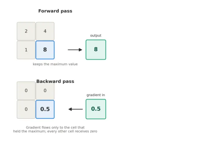
Figure 3. Forward pass keeps the maximum; backward pass routes the gradient only to that cell.

The gradient routing technique clarifies why max pooling does not introduce any trainable weights, since there is nothing for backpropagation to adjust within the layer itself.

Max Pooling in Code

Keras / TensorFlow Example

The MaxPooling2D layer in Keras applies a 2×2 window with a stride of 2 by default.

from tensorflow.keras.layers import MaxPooling2Dimport numpy as np feature_map = np.array([    [2, 4, 7, 5],    [1, 8, 3, 6],    [9, 2, 4, 1],    [3, 7, 5, 8]]).reshape(1, 4, 4, 1) max_pool = MaxPooling2D(pool_size=(2, 2), strides=2)output = max_pool(feature_map) print(output.numpy().reshape(2, 2))

Output:

PyTorch Example

PyTorch implements the same functionality using nn.MaxPool2d. This is the framework currently used in the majority of CNN studies, and this particular framework is missing in all of this article’s competitor sources.

import torchimport torch.nn as nn feature_map = torch.tensor([    [2., 4, 7, 5],    [1, 8, 3, 6],    [9, 2, 4, 1],    [3, 7, 5, 8]]).reshape(1, 1, 4, 4) max_pool = nn.MaxPool2d(kernel_size=2, stride=2)output = max_pool(feature_map) print(output.reshape(2, 2))

Output:

This is because both are essentially carrying out the same operation underneath. The difference in syntax is in that Keras uses pool_size and strides whereas PyTorch uses kernel_size and stride.

Is Max Pooling Still Used in 2026?

However, despite still being utilized, the importance of max pooling in designing CNNs has decreased since 2012.

Max pooling was implemented by Krizhevsky, Sutskever, and Hinton in the architecture of AlexNet, the CNN that emerged victorious at the ILSVRC in 2012. As a result, max pooling became an integral part of the CNNs designed thereafter, including VGG and early versions of ResNets.

Figure 4. Pooling’s role in downsampling has narrowed as architectures moved from LeNet to Vision Transformers.

There are two trends that have made max pooling rarer in new architectures.

• Strided convolutions. Strided convolution is a type of convolution with a stride greater than 1, which down-samples and extracts features at once through a single trainable step. Springenberg et al. (2014) suggested replacing pooling layers with strided convolutions in the “All Convolutional Net” architecture, asserting that a trainable down-sampling operation could outperform a non-trainable one.
• Vision Transformers (ViT). The Vision Transformer uses the self-attention mechanism and treats an image as a sequence of patches without pooling layers.

Max pooling continues to be used in lightweight and edge CNNs due to its inability to have any trainable parameters and keep the model compact and efficient. Max pooling is also a standard practice in training CNN architectures and in mobile optimized CNNs in which every parameter costs.

Choosing Pool Size and Stride

There are three key elements that affect the right pool size and stride for a particular layer.

1. Initially, a 2×2 window and stride of 2 should be taken into account. This setup is utilized in AlexNet, VGG, and most basic CNN tutorials, reducing spatial dimensions twice per layer.
2. Increase the window size only in cases of heavy downsampling. If a window size of 3×3 or greater is taken into account, more spatial information will be lost per layer, which is acceptable only when the input size is relatively high compared to the target size.
3. Make sure that the stride is equal to the window size for non-overlapping pooling. The stride less than the window size will result in overlapping windows, which were initially used in such neural networks as AlexNet to minimize information loss.

FAQs

Conclusion

Pooling operations like max pooling involve selecting only the largest elements from the feature maps based on a comparison that doesn’t require any parameters, and all gradients generated go through one cell in each window that contains the maximum. This process of selection, elimination, and routing of gradients to the winners is the reason why the max pooling is still used in architecture designs up to 2026 for fast and efficient edge computing.